Benchmark DUACS sea surface height maps

2023-04-27 DUACS_SSH_BENCHMARK_DEMO

---

Authors: CLS & Datlas Copyright: 2023 CLS & Datlas License: MIT

Benchmark of DUACS sea surface height maps

The notebook aims to evaluate the sea surface height maps produced by the DUACS system.

<h5> These maps are equivalent to the SEALEVEL_GLO_PHY_L4_MY_008_047 product distributed by the Copernicus Marine Service, except that a nadir altimeter (SARAL/Altika, SEALEVEL_GLO_PHY_L3_MY_008_062 product) has been excluded from the mapping. </h5>
    <h5> We provide below a demonstration of the validation of these maps against the independent SSH data from the Saral/AltiKa altimeter distributed by CMEMS </h5>

---

General Note 1: Execute each cell through the button from the top MENU (or keyboard shortcut Shift + Enter). General Note 2: If, for any reason, the kernel is not working anymore, in the top MENU, click on the button. Then, in the top MENU, click on “Cell” and select “Run All Above Selected Cell”. ***

Learning outcomes

At the end of this notebook you will know:

• How you can evaluated sea surface height maps with independent alongtrack data: statistical and spectral analysis

from glob import glob
import numpy as np
import os

import sys
sys.path.append('..')
from src.mod_plot import *
from src.mod_stat import *
from src.mod_spectral import *

import logging
logger = logging.getLogger()
logger.setLevel(logging.INFO)

0. Parameters

time_min = '2019-01-01'                                        # time min for analysis
time_max = '2019-12-31'                                        # time max for analysis
output_dir = '../results'                                      # output directory path
os.system(f'mkdir -p {output_dir}')
method_name = 'DUACS'
stat_output_filename = f'{output_dir}/stat_sla_duacs_geos.nc'  # output statistical analysis filename
lambda_min = 65.                                               # minimun spatial scale in kilometer to consider on the filtered signal
lambda_max = 500.                                              # maximum spatial scale in kilometer to consider on the filtered signal
psd_output_filename = f'{output_dir}/psd_sla_duacs_geos.nc'    # output spectral analysis filename
segment_lenght = 1000.                                         # spectral parameer: along-track segment lenght in kilometer to consider in the spectral analysis

1. Input files

Sea Surface Height from Saral/AltiKa

%%time
list_of_file = sorted(glob('../data/independent_alongtrack/alg/2019/*.nc'))
ds_alg = xr.open_mfdataset(list_of_file, combine='nested', concat_dim='time')
ds_alg = ds_alg.where((ds_alg.time >= np.datetime64(time_min)) & (ds_alg.time <=  np.datetime64(time_max)), drop=True)
ds_alg = ds_alg.sortby('time')
ds_alg

CPU times: user 52.5 s, sys: 6.28 s, total: 58.8 s
Wall time: 1min 3s

<xarray.Dataset>
Dimensions:         (time: 14437696)
Coordinates:
  * time            (time) datetime64[ns] 2019-01-01T00:04:07.003014144 ... 2...
    longitude       (time) float64 dask.array<chunksize=(44621,), meta=np.ndarray>
    latitude        (time) float64 dask.array<chunksize=(44621,), meta=np.ndarray>
Data variables:
    cycle           (time) float64 dask.array<chunksize=(44621,), meta=np.ndarray>
    track           (time) float64 dask.array<chunksize=(44621,), meta=np.ndarray>
    sla_unfiltered  (time) float32 dask.array<chunksize=(44621,), meta=np.ndarray>
    sla_filtered    (time) float32 dask.array<chunksize=(44621,), meta=np.ndarray>
    dac             (time) float32 dask.array<chunksize=(44621,), meta=np.ndarray>
    ocean_tide      (time) float32 dask.array<chunksize=(44621,), meta=np.ndarray>
    internal_tide   (time) float32 dask.array<chunksize=(44621,), meta=np.ndarray>
    lwe             (time) float32 dask.array<chunksize=(44621,), meta=np.ndarray>
    mdt             (time) float32 dask.array<chunksize=(44621,), meta=np.ndarray>
    tpa_correction  (time) float32 0.0 0.0 0.0 0.0 0.0 ... 0.0 0.0 0.0 0.0 0.0
Attributes: (12/44)
    Conventions:                     CF-1.6
    Metadata_Conventions:            Unidata Dataset Discovery v1.0
    cdm_data_type:                   Swath
    comment:                         Sea surface height measured by altimeter...
    contact:                         servicedesk.cmems@mercator-ocean.eu
    creator_email:                   servicedesk.cmems@mercator-ocean.eu
    ...                              ...
    summary:                         SSALTO/DUACS Delayed-Time Level-3 sea su...
    time_coverage_duration:          P24H11M29.716548S
    time_coverage_end:               2019-01-01T23:36:52Z
    time_coverage_resolution:        P1S
    time_coverage_start:             2018-12-31T23:25:22Z
    title:                           DT Altika Drifting Phase Global Ocean Al...

xarray.Dataset

• Dimensions:
  • time: 14437696
• Coordinates: (3)
  • time
    (time)
    datetime64[ns]
    2019-01-01T00:04:07.003014144 .....

    axis :

    T

    long_name :

    Time of measurement

    standard_name :

    time

    array(['2019-01-01T00:04:07.003014144', '2019-01-01T00:04:08.059014400',
           '2019-01-01T00:04:09.115014144', ..., '2019-12-30T23:56:54.874210816',
           '2019-12-30T23:56:55.930211072', '2019-12-30T23:57:00.154210816'],
          dtype='datetime64[ns]')

  • longitude
    (time)
    float64
    dask.array<chunksize=(44621,), meta=np.ndarray>

    long_name :

    Longitude of measurement

    standard_name :

    longitude

    units :

    degrees_east

    Array Chunk Bytes 110.15 MiB 368.37 kiB Shape (14437696,) (47151,) Dask graph 371 chunks in 733 graph layers Data type float64 numpy.ndarray

  • latitude
    (time)
    float64
    dask.array<chunksize=(44621,), meta=np.ndarray>

    long_name :

    Latitude of measurement

    standard_name :

    latitude

    units :

    degrees_north

    Array Chunk Bytes 110.15 MiB 368.37 kiB Shape (14437696,) (47151,) Dask graph 371 chunks in 733 graph layers Data type float64 numpy.ndarray

• Data variables: (10)
  • cycle
    (time)
    float64
    dask.array<chunksize=(44621,), meta=np.ndarray>

    long_name :

    Cycle the measurement belongs to

    units :

    1

    Array Chunk Bytes 110.15 MiB 368.37 kiB Shape (14437696,) (47151,) Dask graph 371 chunks in 737 graph layers Data type float64 numpy.ndarray

  • track
    (time)
    float64
    dask.array<chunksize=(44621,), meta=np.ndarray>

    long_name :

    Track in cycle the measurement belongs to

    units :

    1

    Array Chunk Bytes 110.15 MiB 368.37 kiB Shape (14437696,) (47151,) Dask graph 371 chunks in 737 graph layers Data type float64 numpy.ndarray

  • sla_unfiltered
    (time)
    float32
    dask.array<chunksize=(44621,), meta=np.ndarray>

    comment :

    The sea level anomaly is the sea surface height above mean sea surface height; the uncorrected sla can be computed as follows: [uncorrected sla]=[sla from product]+[dac]+[ocean_tide]+[internal_tide]-[lwe]; see the product user manual for details

    long_name :

    Sea level anomaly not-filtered not-subsampled with dac, ocean_tide and lwe correction applied

    standard_name :

    sea_surface_height_above_sea_level

    units :

    m

    Array Chunk Bytes 55.08 MiB 184.18 kiB Shape (14437696,) (47151,) Dask graph 371 chunks in 736 graph layers Data type float32 numpy.ndarray

  • sla_filtered
    (time)
    float32
    dask.array<chunksize=(44621,), meta=np.ndarray>

    comment :

    The sea level anomaly is the sea surface height above mean sea surface height; the uncorrected sla can be computed as follows: [uncorrected sla]=[sla from product]+[dac]+[ocean_tide]+[internal_tide]-[lwe]; see the product user manual for details

    long_name :

    Sea level anomaly filtered not-subsampled with dac, ocean_tide and lwe correction applied

    standard_name :

    sea_surface_height_above_sea_level

    units :

    m

    Array Chunk Bytes 55.08 MiB 184.18 kiB Shape (14437696,) (47151,) Dask graph 371 chunks in 736 graph layers Data type float32 numpy.ndarray

  • dac
    (time)
    float32
    dask.array<chunksize=(44621,), meta=np.ndarray>

    comment :

    The sla in this file is already corrected for the dac; the uncorrected sla can be computed as follows: [uncorrected sla]=[sla from product]+[dac]; see the product user manual for details

    long_name :

    Dynamic Atmospheric Correction

    units :

    m

    Array Chunk Bytes 55.08 MiB 184.18 kiB Shape (14437696,) (47151,) Dask graph 371 chunks in 736 graph layers Data type float32 numpy.ndarray

  • ocean_tide
    (time)
    float32
    dask.array<chunksize=(44621,), meta=np.ndarray>

    comment :

    The sla in this file is already corrected for the ocean_tide; the uncorrected sla can be computed as follows: [uncorrected sla]=[sla from product]+[ocean_tide]; see the product user manual for details

    long_name :

    Ocean tide model

    units :

    m

    Array Chunk Bytes 55.08 MiB 184.18 kiB Shape (14437696,) (47151,) Dask graph 371 chunks in 736 graph layers Data type float32 numpy.ndarray

  • internal_tide
    (time)
    float32
    dask.array<chunksize=(44621,), meta=np.ndarray>

    comment :

    The sla in this file is already corrected for the internal_tide; the uncorrected sla can be computed as follows: [uncorrected sla]=[sla from product]+[internal_tide]; see the product user manual for details

    long_name :

    Internal tide correction

    units :

    m

    Array Chunk Bytes 55.08 MiB 184.18 kiB Shape (14437696,) (47151,) Dask graph 371 chunks in 736 graph layers Data type float32 numpy.ndarray

  • lwe
    (time)
    float32
    dask.array<chunksize=(44621,), meta=np.ndarray>

    comment :

    The sla in this file is already corrected for the lwe; the uncorrected sla can be computed as follows: [uncorrected sla]=[sla from product]-[lwe]; see the product user manual for details

    long_name :

    Long wavelength error

    units :

    m

    Array Chunk Bytes 55.08 MiB 184.18 kiB Shape (14437696,) (47151,) Dask graph 371 chunks in 736 graph layers Data type float32 numpy.ndarray

  • mdt
    (time)
    float32
    dask.array<chunksize=(44621,), meta=np.ndarray>

    comment :

    The mean dynamic topography is the sea surface height above geoid; it is used to compute the absolute dynamic tyopography adt=sla+mdt

    long_name :

    Mean dynamic topography

    standard_name :

    sea_surface_height_above_geoid

    units :

    m

    Array Chunk Bytes 55.08 MiB 184.18 kiB Shape (14437696,) (47151,) Dask graph 371 chunks in 736 graph layers Data type float32 numpy.ndarray

  • tpa_correction
    (time)
    float32
    0.0 0.0 0.0 0.0 ... 0.0 0.0 0.0 0.0

    comment :

    This variable can be added to the SLA to correct for the observed instrumental drift during the lifetime of the TOPEX-A mission (the correction is null after this period). This is a global correction to be added a posteriori (and not before) on the global mean sea level estimate derived from the along-track product. It can be applied at regional or local scale as a best estimate (better than no correction, since the regional variation of the instrumental drift is unknown). See product manual for more details.

    long_name :

    TOPEX-A instrumental drift correction derived from altimetry and tide gauges global comparisons (WCRP Sea Level Budget Group, 2018)

    standard_name :

    sea_surface_height_above_sea_level

    units :

    m

    array([0., 0., 0., ..., 0., 0., 0.], dtype=float32)

• Indexes: (1)
  • time
    PandasIndex

    PandasIndex(DatetimeIndex(['2019-01-01 00:04:07.003014144',
                   '2019-01-01 00:04:08.059014400',
                   '2019-01-01 00:04:09.115014144',
                   '2019-01-01 00:04:11.227014144',
                   '2019-01-01 00:04:12.283014144',
                   '2019-01-01 00:04:13.339014144',
                   '2019-01-01 00:04:14.395014144',
                   '2019-01-01 00:04:15.451014400',
                   '2019-01-01 00:04:16.507013888',
                   '2019-01-01 00:04:17.563014144',
                   ...
                   '2019-12-30 23:56:47.482210816',
                   '2019-12-30 23:56:48.538211072',
                   '2019-12-30 23:56:49.594211072',
                   '2019-12-30 23:56:50.650211072',
                   '2019-12-30 23:56:51.706210816',
                   '2019-12-30 23:56:52.762210816',
                   '2019-12-30 23:56:53.818210816',
                   '2019-12-30 23:56:54.874210816',
                   '2019-12-30 23:56:55.930211072',
                   '2019-12-30 23:57:00.154210816'],
                  dtype='datetime64[ns]', name='time', length=14437696, freq=None))

• Attributes: (44)

  Conventions :

  CF-1.6

  Metadata_Conventions :

  Unidata Dataset Discovery v1.0

  cdm_data_type :

  Swath

  comment :

  Sea surface height measured by altimeters referenced to the [1993, 2012] period; with additional corrections; the proposed sla is already corrected for dac, ocean_tide and lwe; [uncorrected sla]=[sla from product]+[dac]+[ocean_tide]-[lwe]

  contact :

  servicedesk.cmems@mercator-ocean.eu

  creator_email :

  servicedesk.cmems@mercator-ocean.eu

  creator_name :

  CMEMS - Sea Level Thematic Assembly Center

  creator_url :

  http://marine.copernicus.eu

  date_created :

  2021-09-08T13:54:51Z

  date_issued :

  2021-09-08T13:54:51Z

  date_modified :

  2021-09-08T13:54:51Z

  geospatial_lat_max :

  81.443179

  geospatial_lat_min :

  -78.158928

  geospatial_lat_resolution :

  0.0556490000000025

  geospatial_lat_units :

  degrees_north

  geospatial_lon_max :

  359.998793

  geospatial_lon_min :

  0.010756

  geospatial_lon_resolution :

  0.017816999999979544

  geospatial_lon_units :

  degrees_east

  geospatial_vertical_max :

  0.0

  geospatial_vertical_min :

  0.0

  geospatial_vertical_positive :

  down

  geospatial_vertical_resolution :

  point

  geospatial_vertical_units :

  m

  history :

  2021-09-08T13:54:51Z: Creation

  institution :

  CLS, CNES

  keywords :

  Oceans > Ocean Topography > Sea Surface Height

  keywords_vocabulary :

  NetCDF COARDS Climate and Forecast Standard Names

  license :

  http://marine.copernicus.eu/web/27-service-commitments-and-licence.php

  platform :

  Altika Drifting Phase

  processing_level :

  L3

  product_version :

  vDec2021

  project :

  COPERNICUS MARINE ENVIRONMENT MONITORING SERVICE (CMEMS)

  references :

  http://marine.copernicus.eu

  software_version :

  7.0_DUACS_DT2021_baseline

  source :

  Altika Drifting Phase measurements

  ssalto_duacs_comment :

  The reference mission used for the altimeter inter-calibration processing is Topex/Poseidon between 1993-01-01 and 2002-04-23, Jason-1 between 2002-04-24 and 2008-10-18, OSTM/Jason-2 between 2008-10-19 and 2016-06-25, Jason-3 since 2016-06-25.

  standard_name_vocabulary :

  NetCDF Climate and Forecast (CF) Metadata Convention Standard Name Table v37

  summary :

  SSALTO/DUACS Delayed-Time Level-3 sea surface height measured by Altika Drifting Phase altimetry observations over Global Ocean.

  time_coverage_duration :

  P24H11M29.716548S

  time_coverage_end :

  2019-01-01T23:36:52Z

  time_coverage_resolution :

  P1S

  time_coverage_start :

  2018-12-31T23:25:22Z

  title :

  DT Altika Drifting Phase Global Ocean Along track SSALTO/DUACS Sea Surface Height L3 product

Sea Surface Height maps to evaluate

%%time
list_of_maps = sorted(glob('../data/maps/DUACS_global_allsat-alg/*.nc'))
ds_maps = xr.open_mfdataset(list_of_maps, combine='nested', concat_dim='time')
ds_maps = ds_maps.sel(time=slice(time_min, time_max))
ds_maps

CPU times: user 6.2 s, sys: 741 ms, total: 6.94 s
Wall time: 8.42 s

<xarray.Dataset>
Dimensions:    (latitude: 720, longitude: 1440, time: 365)
Coordinates:
  * latitude   (latitude) float32 -89.88 -89.62 -89.38 ... 89.38 89.62 89.88
  * longitude  (longitude) float64 0.125 0.375 0.625 0.875 ... 359.4 359.6 359.9
  * time       (time) datetime64[ns] 2019-01-01 2019-01-02 ... 2019-12-31
Data variables:
    sla        (time, latitude, longitude) float64 dask.array<chunksize=(1, 720, 1440), meta=np.ndarray>
    ugosa      (time, latitude, longitude) float64 dask.array<chunksize=(1, 720, 1440), meta=np.ndarray>
    vgosa      (time, latitude, longitude) float64 dask.array<chunksize=(1, 720, 1440), meta=np.ndarray>
    adt        (time, latitude, longitude) float64 dask.array<chunksize=(1, 720, 1440), meta=np.ndarray>
    ugos       (time, latitude, longitude) float64 dask.array<chunksize=(1, 720, 1440), meta=np.ndarray>
    vgos       (time, latitude, longitude) float64 dask.array<chunksize=(1, 720, 1440), meta=np.ndarray>

xarray.Dataset

• Dimensions:
  • latitude: 720
  • longitude: 1440
  • time: 365
• Coordinates: (3)
  • latitude
    (latitude)
    float32
    -89.88 -89.62 ... 89.62 89.88

    axis :

    Y

    bounds :

    lat_bnds

    long_name :

    Latitude

    standard_name :

    latitude

    units :

    degrees_north

    valid_max :

    89.875

    valid_min :

    -89.875

    array([-89.875, -89.625, -89.375, ...,  89.375,  89.625,  89.875],
          dtype=float32)

  • longitude
    (longitude)
    float64
    0.125 0.375 0.625 ... 359.6 359.9

    valid_max :

    359.875

    valid_min :

    0.125

    bounds :

    lon_bnds

    axis :

    X

    long_name :

    Longitude

    standard_name :

    longitude

    units :

    degrees_east

    array([1.25000e-01, 3.75000e-01, 6.25000e-01, ..., 3.59375e+02, 3.59625e+02,
           3.59875e+02])

  • time
    (time)
    datetime64[ns]
    2019-01-01 ... 2019-12-31

    axis :

    T

    long_name :

    Time

    standard_name :

    time

    array(['2019-01-01T00:00:00.000000000', '2019-01-02T00:00:00.000000000',
           '2019-01-03T00:00:00.000000000', ..., '2019-12-29T00:00:00.000000000',
           '2019-12-30T00:00:00.000000000', '2019-12-31T00:00:00.000000000'],
          dtype='datetime64[ns]')

• Data variables: (6)
  • sla
    (time, latitude, longitude)
    float64
    dask.array<chunksize=(1, 720, 1440), meta=np.ndarray>

    ancillary_variables :

    err_sla

    comment :

    The sea level anomaly is the sea surface height above mean sea surface; it is referenced to the [1993, 2012] period; see the product user manual for details

    grid_mapping :

    crs

    long_name :

    Sea level anomaly

    standard_name :

    sea_surface_height_above_sea_level

    units :

    m

    Array Chunk Bytes 2.82 GiB 7.91 MiB Shape (365, 720, 1440) (1, 720, 1440) Dask graph 365 chunks in 731 graph layers Data type float64 numpy.ndarray

  • ugosa
    (time, latitude, longitude)
    float64
    dask.array<chunksize=(1, 720, 1440), meta=np.ndarray>

    ancillary_variables :

    err_ugosa

    comment :

    The geostrophic velocity anomalies are referenced to the [1993, 2012] period

    grid_mapping :

    crs

    long_name :

    Geostrophic velocity anomalies: zonal component

    standard_name :

    surface_geostrophic_eastward_sea_water_velocity_assuming_sea_level_for_geoid

    units :

    m/s

    Array Chunk Bytes 2.82 GiB 7.91 MiB Shape (365, 720, 1440) (1, 720, 1440) Dask graph 365 chunks in 731 graph layers Data type float64 numpy.ndarray

  • vgosa
    (time, latitude, longitude)
    float64
    dask.array<chunksize=(1, 720, 1440), meta=np.ndarray>

    ancillary_variables :

    err_vgosa

    comment :

    The geostrophic velocity anomalies are referenced to the [1993, 2012] period

    grid_mapping :

    crs

    long_name :

    Geostrophic velocity anomalies: meridian component

    standard_name :

    surface_geostrophic_northward_sea_water_velocity_assuming_sea_level_for_geoid

    units :

    m/s

    Array Chunk Bytes 2.82 GiB 7.91 MiB Shape (365, 720, 1440) (1, 720, 1440) Dask graph 365 chunks in 731 graph layers Data type float64 numpy.ndarray

  • adt
    (time, latitude, longitude)
    float64
    dask.array<chunksize=(1, 720, 1440), meta=np.ndarray>

    comment :

    The absolute dynamic topography is the sea surface height above geoid; the adt is obtained as follows: adt=sla+mdt where mdt is the mean dynamic topography; see the product user manual for details

    grid_mapping :

    crs

    long_name :

    Absolute dynamic topography

    standard_name :

    sea_surface_height_above_geoid

    units :

    m

    Array Chunk Bytes 2.82 GiB 7.91 MiB Shape (365, 720, 1440) (1, 720, 1440) Dask graph 365 chunks in 731 graph layers Data type float64 numpy.ndarray

  • ugos
    (time, latitude, longitude)
    float64
    dask.array<chunksize=(1, 720, 1440), meta=np.ndarray>

    grid_mapping :

    crs

    long_name :

    Absolute geostrophic velocity: zonal component

    standard_name :

    surface_geostrophic_eastward_sea_water_velocity

    units :

    m/s

    Array Chunk Bytes 2.82 GiB 7.91 MiB Shape (365, 720, 1440) (1, 720, 1440) Dask graph 365 chunks in 731 graph layers Data type float64 numpy.ndarray

  • vgos
    (time, latitude, longitude)
    float64
    dask.array<chunksize=(1, 720, 1440), meta=np.ndarray>

    grid_mapping :

    crs

    long_name :

    Absolute geostrophic velocity: meridian component

    standard_name :

    surface_geostrophic_northward_sea_water_velocity

    units :

    m/s

    Array Chunk Bytes 2.82 GiB 7.91 MiB Shape (365, 720, 1440) (1, 720, 1440) Dask graph 365 chunks in 731 graph layers Data type float64 numpy.ndarray

• Indexes: (3)
  • latitude
    PandasIndex

    PandasIndex(Float64Index([-89.875, -89.625, -89.375, -89.125, -88.875, -88.625, -88.375,
                  -88.125, -87.875, -87.625,
                  ...
                   87.625,  87.875,  88.125,  88.375,  88.625,  88.875,  89.125,
                   89.375,  89.625,  89.875],
                 dtype='float64', name='latitude', length=720))

  • longitude
    PandasIndex

    PandasIndex(Float64Index([  0.125,   0.375,   0.625,   0.875,   1.125,   1.375,   1.625,
                    1.875,   2.125,   2.375,
                  ...
                  357.625, 357.875, 358.125, 358.375, 358.625, 358.875, 359.125,
                  359.375, 359.625, 359.875],
                 dtype='float64', name='longitude', length=1440))

  • time
    PandasIndex

    PandasIndex(DatetimeIndex(['2019-01-01', '2019-01-02', '2019-01-03', '2019-01-04',
                   '2019-01-05', '2019-01-06', '2019-01-07', '2019-01-08',
                   '2019-01-09', '2019-01-10',
                   ...
                   '2019-12-22', '2019-12-23', '2019-12-24', '2019-12-25',
                   '2019-12-26', '2019-12-27', '2019-12-28', '2019-12-29',
                   '2019-12-30', '2019-12-31'],
                  dtype='datetime64[ns]', name='time', length=365, freq=None))

• Attributes: (0)

2. Statistical & Spectral Analysis

2.1 Interpolate sea surface height maps onto along-track positions

ds_interp = run_interpolation(ds_maps, ds_alg)
ds_interp = ds_interp.dropna('time')
ds_interp

2023-07-07 16:55:04 INFO     fetch data from 2019-01-01 00:00:00 to 2019-02-01 00:00:00
2023-07-07 16:55:06 INFO     fetch data from 2019-01-31 00:00:00 to 2019-03-01 00:00:00
2023-07-07 16:55:09 INFO     fetch data from 2019-02-28 00:00:00 to 2019-04-01 00:00:00
2023-07-07 16:55:11 INFO     fetch data from 2019-03-31 00:00:00 to 2019-05-01 00:00:00
2023-07-07 16:55:13 INFO     fetch data from 2019-04-30 00:00:00 to 2019-06-01 00:00:00
2023-07-07 16:55:16 INFO     fetch data from 2019-05-31 00:00:00 to 2019-07-01 00:00:00
2023-07-07 16:55:18 INFO     fetch data from 2019-06-30 00:00:00 to 2019-08-01 00:00:00
2023-07-07 16:55:20 INFO     fetch data from 2019-07-31 00:00:00 to 2019-09-01 00:00:00
2023-07-07 16:55:23 INFO     fetch data from 2019-08-31 00:00:00 to 2019-10-01 00:00:00
2023-07-07 16:55:25 INFO     fetch data from 2019-09-30 00:00:00 to 2019-11-01 00:00:00
2023-07-07 16:55:28 INFO     fetch data from 2019-10-31 00:00:00 to 2019-12-01 00:00:00
2023-07-07 16:55:30 INFO     fetch data from 2019-11-30 00:00:00 to 2019-12-31 00:00:00

<xarray.Dataset>
Dimensions:            (time: 14348023)
Coordinates:
  * time               (time) datetime64[ns] 2019-01-01T00:04:07.003014144 .....
Data variables: (12/13)
    cycle              (time) float64 126.0 126.0 126.0 ... 136.0 136.0 136.0
    track              (time) float64 9.0 9.0 9.0 9.0 ... 408.0 408.0 408.0
    sla_unfiltered     (time) float32 0.127 0.101 0.07 ... 0.007 0.056 0.01
    sla_filtered       (time) float32 0.117 0.128 0.142 ... 0.03 0.031 0.027
    dac                (time) float32 0.303 0.299 0.296 ... 0.172 0.171 0.172
    ocean_tide         (time) float32 -0.091 -0.096 -0.099 ... -0.304 -0.314
    ...                 ...
    lwe                (time) float32 -0.019 -0.019 -0.019 ... 0.014 0.014 0.016
    mdt                (time) float32 -0.104 -0.106 -0.108 ... -1.138 -1.154
    tpa_correction     (time) float32 0.0 0.0 0.0 0.0 0.0 ... 0.0 0.0 0.0 0.0
    longitude          (time) float64 64.42 64.33 64.25 ... 246.7 246.6 246.3
    latitude           (time) float64 69.9 69.95 70.01 ... -69.27 -69.32 -69.55
    msla_interpolated  (time) float64 0.1568 0.1544 0.1564 ... 0.0136 0.02117

xarray.Dataset

• Dimensions:
  • time: 14348023
• Coordinates: (1)
  • time
    (time)
    datetime64[ns]
    2019-01-01T00:04:07.003014144 .....

    array(['2019-01-01T00:04:07.003014144', '2019-01-01T00:04:08.059014400',
           '2019-01-01T00:04:09.115014144', ..., '2019-12-30T23:56:54.874210816',
           '2019-12-30T23:56:55.930211072', '2019-12-30T23:57:00.154210816'],
          dtype='datetime64[ns]')

• Data variables: (13)
  • cycle
    (time)
    float64
    126.0 126.0 126.0 ... 136.0 136.0

    array([126., 126., 126., ..., 136., 136., 136.])

  • track
    (time)
    float64
    9.0 9.0 9.0 ... 408.0 408.0 408.0

    array([  9.,   9.,   9., ..., 408., 408., 408.])

  • sla_unfiltered
    (time)
    float32
    0.127 0.101 0.07 ... 0.056 0.01

    array([0.127, 0.101, 0.07 , ..., 0.007, 0.056, 0.01 ], dtype=float32)

  • sla_filtered
    (time)
    float32
    0.117 0.128 0.142 ... 0.031 0.027

    array([0.11700001, 0.128     , 0.142     , ..., 0.03      , 0.031     ,
           0.027     ], dtype=float32)

  • dac
    (time)
    float32
    0.303 0.299 0.296 ... 0.171 0.172

    array([0.303     , 0.29900002, 0.296     , ..., 0.172     , 0.171     ,
           0.172     ], dtype=float32)

  • ocean_tide
    (time)
    float32
    -0.091 -0.096 ... -0.304 -0.314

    array([-0.09100001, -0.096     , -0.09900001, ..., -0.30100003,
           -0.30400002, -0.314     ], dtype=float32)

  • internal_tide
    (time)
    float32
    0.0 0.0 0.0 0.0 ... 0.0 0.0 0.0 0.0

    array([0., 0., 0., ..., 0., 0., 0.], dtype=float32)

  • lwe
    (time)
    float32
    -0.019 -0.019 ... 0.014 0.016

    array([-0.019, -0.019, -0.019, ...,  0.014,  0.014,  0.016], dtype=float32)

  • mdt
    (time)
    float32
    -0.104 -0.106 ... -1.138 -1.154

    array([-0.104     , -0.10600001, -0.108     , ..., -1.136     ,
           -1.138     , -1.154     ], dtype=float32)

  • tpa_correction
    (time)
    float32
    0.0 0.0 0.0 0.0 ... 0.0 0.0 0.0 0.0

    array([0., 0., 0., ..., 0., 0., 0.], dtype=float32)

  • longitude
    (time)
    float64
    64.42 64.33 64.25 ... 246.6 246.3

    array([ 64.416461,  64.334183,  64.251484, ..., 246.653539, 246.574455,
           246.254122])

  • latitude
    (time)
    float64
    69.9 69.95 70.01 ... -69.32 -69.55

    array([ 69.897148,  69.953286,  70.009389, ..., -69.265878, -69.32329 ,
           -69.552607])

  • msla_interpolated
    (time)
    float64
    0.1568 0.1544 ... 0.0136 0.02117

    array([0.15677194, 0.15439134, 0.15639504, ..., 0.01124466, 0.01359573,
           0.02117254])

• Indexes: (1)
  • time
    PandasIndex

    PandasIndex(DatetimeIndex(['2019-01-01 00:04:07.003014144',
                   '2019-01-01 00:04:08.059014400',
                   '2019-01-01 00:04:09.115014144',
                   '2019-01-01 00:04:11.227014144',
                   '2019-01-01 00:04:12.283014144',
                   '2019-01-01 00:04:13.339014144',
                   '2019-01-01 00:04:14.395014144',
                   '2019-01-01 00:04:15.451014400',
                   '2019-01-01 00:04:16.507013888',
                   '2019-01-01 00:04:17.563014144',
                   ...
                   '2019-12-30 23:56:47.482210816',
                   '2019-12-30 23:56:48.538211072',
                   '2019-12-30 23:56:49.594211072',
                   '2019-12-30 23:56:50.650211072',
                   '2019-12-30 23:56:51.706210816',
                   '2019-12-30 23:56:52.762210816',
                   '2019-12-30 23:56:53.818210816',
                   '2019-12-30 23:56:54.874210816',
                   '2019-12-30 23:56:55.930211072',
                   '2019-12-30 23:57:00.154210816'],
                  dtype='datetime64[ns]', name='time', length=14348023, freq=None))

• Attributes: (0)

2.2 Compute grid boxes statistics & statistics by regime (coastal, offshore low variability, offshore high variability)

Once the maps have been interpolated to the position of the along-track, it is possible to calculate different statistics on the time series SLA_alongtrack and SLA_maps.

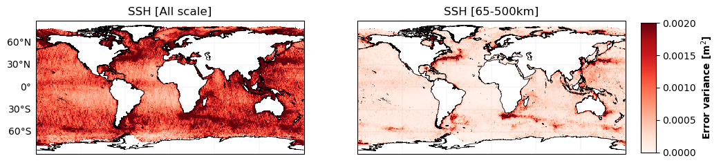
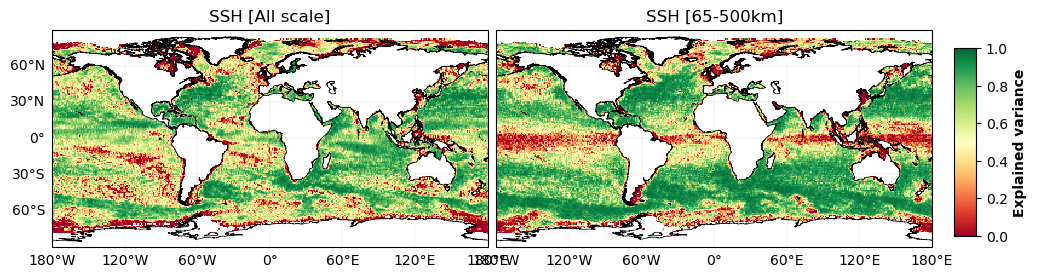
We propose below the following statistics: error variance maps (static by 1°x1° box), explained variance maps, temporal evolution of global error variance and explained variance.

These statistics are also applied to the filtered signals focusing on the 65-500km scale range. A bandpass filter is applied before calculating the scores.

compute_stat_scores(ds_interp, lambda_min, lambda_max, stat_output_filename,method_name)

2023-07-07 16:58:30 INFO     Compute mapping error all scales
2023-07-07 16:58:31 INFO     Compute mapping error for scales between 65.0 and 500.0 km
2023-07-07 16:59:49 INFO     Compute binning statistics
2023-07-07 17:00:09 INFO     Compute statistics by oceanic regime
2023-07-07 17:01:03 INFO     Stat file saved as: ../results/stat_sla_duacs_geos.nc

# Plot gridded stats
# Hvplot
# plot_stat_score_map(stat_output_filename)
# Matplotlib
plot_stat_score_map_png(stat_output_filename)

plot_stat_score_timeseries(stat_output_filename)

plot_stat_by_regimes(stat_output_filename)

	mapping_err_var [m²]	sla_unfiltered_var [m²]	mapping_err_filtered_var [m²]	sla_filtered_var [m²]	var_score_allscale	var_score_filtered
coastal	0.002611	0.008254	0.000572	0.001804	0.683678	0.682788
offshore_highvar	0.003125	0.053255	0.001055	0.021749	0.941316	0.951509
offshore_lowvar	0.001258	0.006296	0.000234	0.001775	0.800111	0.868348
equatorial_band	0.001404	0.005963	0.000311	0.000533	0.764560	0.415881
arctic	0.002303	0.006915	0.000417	0.001006	0.667031	0.585653
antarctic	0.003287	0.002323	0.000696	0.000754	-0.415025	0.077469

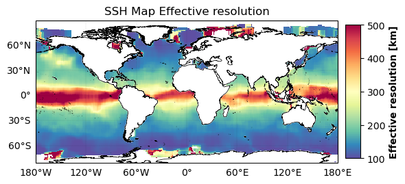
2.3 Compute Spectral scores

compute_psd_scores_v2(ds_interp, psd_output_filename, lenght_scale=segment_lenght,method_name=method_name)

2023-07-05 17:03:17 INFO     Segment computation...
2023-07-05 17:03:33 INFO     Spectral analysis...
2023-07-05 17:19:27 INFO     Saving ouput...
2023-07-05 17:19:35 INFO     PSD file saved as: ../results/psd_sla_duacs_geos.nc

# Plot effective resolution
# Hvplot
# plot_effective_resolution(psd_output_filename)
# Matplotlib
plot_effective_resolution_png(psd_output_filename)

plot_psd_scores(psd_output_filename)

The interactive plot above allows you to explore the spectral metrics by latitude / longitude box