Alongtrack spectral metrics

2023-04-27 DUACS_SSH_BENCHMARK_DEMO

---

Authors: CLS & Datlas Copyright: 2023 CLS & Datlas License: MIT

from glob import glob
import numpy as np
import os

import sys
sys.path.append('..')
from src.mod_plot import *
from src.mod_stat import *
from src.mod_spectral import *

import logging
logger = logging.getLogger()
logger.setLevel(logging.INFO)

0. Parameters

time_min = '2019-01-01'                                        # time min for analysis
time_max = '2019-12-31'                                        # time max for analysis
output_dir = '../results'                                      # output directory path
os.system(f'mkdir -p {output_dir}')
method_name = 'DUACS'
stat_output_filename = f'{output_dir}/stat_sla_duacs_geos.nc'  # output statistical analysis filename
lambda_min = 65.                                               # minimun spatial scale in kilometer to consider on the filtered signal
lambda_max = 500.                                              # maximum spatial scale in kilometer to consider on the filtered signal
psd_output_filename = f'{output_dir}/psd_sla_duacs_geos.nc'    # output spectral analysis filename
segment_lenght = 1000.                                         # spectral parameer: along-track segment lenght in kilometer to consider in the spectral analysis

1. Input files

Sea Surface Height from Saral/AltiKa

%%time
list_of_file = sorted(glob('../data/independent_alongtrack/alg/2019/*.nc'))
ds_alg = xr.open_mfdataset(list_of_file, combine='nested', concat_dim='time')
ds_alg = ds_alg.where((ds_alg.time >= np.datetime64(time_min)) & (ds_alg.time <=  np.datetime64(time_max)), drop=True)
ds_alg = ds_alg.sortby('time')
ds_alg

CPU times: user 52.5 s, sys: 6.28 s, total: 58.8 s
Wall time: 1min 3s

<xarray.Dataset>
Dimensions:         (time: 14437696)
Coordinates:
  * time            (time) datetime64[ns] 2019-01-01T00:04:07.003014144 ... 2...
    longitude       (time) float64 dask.array<chunksize=(44621,), meta=np.ndarray>
    latitude        (time) float64 dask.array<chunksize=(44621,), meta=np.ndarray>
Data variables:
    cycle           (time) float64 dask.array<chunksize=(44621,), meta=np.ndarray>
    track           (time) float64 dask.array<chunksize=(44621,), meta=np.ndarray>
    sla_unfiltered  (time) float32 dask.array<chunksize=(44621,), meta=np.ndarray>
    sla_filtered    (time) float32 dask.array<chunksize=(44621,), meta=np.ndarray>
    dac             (time) float32 dask.array<chunksize=(44621,), meta=np.ndarray>
    ocean_tide      (time) float32 dask.array<chunksize=(44621,), meta=np.ndarray>
    internal_tide   (time) float32 dask.array<chunksize=(44621,), meta=np.ndarray>
    lwe             (time) float32 dask.array<chunksize=(44621,), meta=np.ndarray>
    mdt             (time) float32 dask.array<chunksize=(44621,), meta=np.ndarray>
    tpa_correction  (time) float32 0.0 0.0 0.0 0.0 0.0 ... 0.0 0.0 0.0 0.0 0.0
Attributes: (12/44)
    Conventions:                     CF-1.6
    Metadata_Conventions:            Unidata Dataset Discovery v1.0
    cdm_data_type:                   Swath
    comment:                         Sea surface height measured by altimeter...
    contact:                         servicedesk.cmems@mercator-ocean.eu
    creator_email:                   servicedesk.cmems@mercator-ocean.eu
    ...                              ...
    summary:                         SSALTO/DUACS Delayed-Time Level-3 sea su...
    time_coverage_duration:          P24H11M29.716548S
    time_coverage_end:               2019-01-01T23:36:52Z
    time_coverage_resolution:        P1S
    time_coverage_start:             2018-12-31T23:25:22Z
    title:                           DT Altika Drifting Phase Global Ocean Al...

xarray.Dataset

• Dimensions:
  • time: 14437696
• Coordinates: (3)
  • time
    (time)
    datetime64[ns]
    2019-01-01T00:04:07.003014144 .....

    axis :

    T

    long_name :

    Time of measurement

    standard_name :

    time

    array(['2019-01-01T00:04:07.003014144', '2019-01-01T00:04:08.059014400',
           '2019-01-01T00:04:09.115014144', ..., '2019-12-30T23:56:54.874210816',
           '2019-12-30T23:56:55.930211072', '2019-12-30T23:57:00.154210816'],
          dtype='datetime64[ns]')

  • longitude
    (time)
    float64
    dask.array<chunksize=(44621,), meta=np.ndarray>

    long_name :

    Longitude of measurement

    standard_name :

    longitude

    units :

    degrees_east

    Array Chunk Bytes 110.15 MiB 368.37 kiB Shape (14437696,) (47151,) Dask graph 371 chunks in 733 graph layers Data type float64 numpy.ndarray

  • latitude
    (time)
    float64
    dask.array<chunksize=(44621,), meta=np.ndarray>

    long_name :

    Latitude of measurement

    standard_name :

    latitude

    units :

    degrees_north

    Array Chunk Bytes 110.15 MiB 368.37 kiB Shape (14437696,) (47151,) Dask graph 371 chunks in 733 graph layers Data type float64 numpy.ndarray

• Data variables: (10)
  • cycle
    (time)
    float64
    dask.array<chunksize=(44621,), meta=np.ndarray>

    long_name :

    Cycle the measurement belongs to

    units :

    1

    Array Chunk Bytes 110.15 MiB 368.37 kiB Shape (14437696,) (47151,) Dask graph 371 chunks in 737 graph layers Data type float64 numpy.ndarray

  • track
    (time)
    float64
    dask.array<chunksize=(44621,), meta=np.ndarray>

    long_name :

    Track in cycle the measurement belongs to

    units :

    1

    Array Chunk Bytes 110.15 MiB 368.37 kiB Shape (14437696,) (47151,) Dask graph 371 chunks in 737 graph layers Data type float64 numpy.ndarray

  • sla_unfiltered
    (time)
    float32
    dask.array<chunksize=(44621,), meta=np.ndarray>

    comment :

    The sea level anomaly is the sea surface height above mean sea surface height; the uncorrected sla can be computed as follows: [uncorrected sla]=[sla from product]+[dac]+[ocean_tide]+[internal_tide]-[lwe]; see the product user manual for details

    long_name :

    Sea level anomaly not-filtered not-subsampled with dac, ocean_tide and lwe correction applied

    standard_name :

    sea_surface_height_above_sea_level

    units :

    m

    Array Chunk Bytes 55.08 MiB 184.18 kiB Shape (14437696,) (47151,) Dask graph 371 chunks in 736 graph layers Data type float32 numpy.ndarray

  • sla_filtered
    (time)
    float32
    dask.array<chunksize=(44621,), meta=np.ndarray>

    comment :

    The sea level anomaly is the sea surface height above mean sea surface height; the uncorrected sla can be computed as follows: [uncorrected sla]=[sla from product]+[dac]+[ocean_tide]+[internal_tide]-[lwe]; see the product user manual for details

    long_name :

    Sea level anomaly filtered not-subsampled with dac, ocean_tide and lwe correction applied

    standard_name :

    sea_surface_height_above_sea_level

    units :

    m

    Array Chunk Bytes 55.08 MiB 184.18 kiB Shape (14437696,) (47151,) Dask graph 371 chunks in 736 graph layers Data type float32 numpy.ndarray

  • dac
    (time)
    float32
    dask.array<chunksize=(44621,), meta=np.ndarray>

    comment :

    The sla in this file is already corrected for the dac; the uncorrected sla can be computed as follows: [uncorrected sla]=[sla from product]+[dac]; see the product user manual for details

    long_name :

    Dynamic Atmospheric Correction

    units :

    m

    Array Chunk Bytes 55.08 MiB 184.18 kiB Shape (14437696,) (47151,) Dask graph 371 chunks in 736 graph layers Data type float32 numpy.ndarray

  • ocean_tide
    (time)
    float32
    dask.array<chunksize=(44621,), meta=np.ndarray>

    comment :

    The sla in this file is already corrected for the ocean_tide; the uncorrected sla can be computed as follows: [uncorrected sla]=[sla from product]+[ocean_tide]; see the product user manual for details

    long_name :

    Ocean tide model

    units :

    m

    Array Chunk Bytes 55.08 MiB 184.18 kiB Shape (14437696,) (47151,) Dask graph 371 chunks in 736 graph layers Data type float32 numpy.ndarray

  • internal_tide
    (time)
    float32
    dask.array<chunksize=(44621,), meta=np.ndarray>

    comment :

    The sla in this file is already corrected for the internal_tide; the uncorrected sla can be computed as follows: [uncorrected sla]=[sla from product]+[internal_tide]; see the product user manual for details

    long_name :

    Internal tide correction

    units :

    m

    Array Chunk Bytes 55.08 MiB 184.18 kiB Shape (14437696,) (47151,) Dask graph 371 chunks in 736 graph layers Data type float32 numpy.ndarray

  • lwe
    (time)
    float32
    dask.array<chunksize=(44621,), meta=np.ndarray>

    comment :

    The sla in this file is already corrected for the lwe; the uncorrected sla can be computed as follows: [uncorrected sla]=[sla from product]-[lwe]; see the product user manual for details

    long_name :

    Long wavelength error

    units :

    m

    Array Chunk Bytes 55.08 MiB 184.18 kiB Shape (14437696,) (47151,) Dask graph 371 chunks in 736 graph layers Data type float32 numpy.ndarray

  • mdt
    (time)
    float32
    dask.array<chunksize=(44621,), meta=np.ndarray>

    comment :

    The mean dynamic topography is the sea surface height above geoid; it is used to compute the absolute dynamic tyopography adt=sla+mdt

    long_name :

    Mean dynamic topography

    standard_name :

    sea_surface_height_above_geoid

    units :

    m

    Array Chunk Bytes 55.08 MiB 184.18 kiB Shape (14437696,) (47151,) Dask graph 371 chunks in 736 graph layers Data type float32 numpy.ndarray

  • tpa_correction
    (time)
    float32
    0.0 0.0 0.0 0.0 ... 0.0 0.0 0.0 0.0

    comment :

    This variable can be added to the SLA to correct for the observed instrumental drift during the lifetime of the TOPEX-A mission (the correction is null after this period). This is a global correction to be added a posteriori (and not before) on the global mean sea level estimate derived from the along-track product. It can be applied at regional or local scale as a best estimate (better than no correction, since the regional variation of the instrumental drift is unknown). See product manual for more details.

    long_name :

    TOPEX-A instrumental drift correction derived from altimetry and tide gauges global comparisons (WCRP Sea Level Budget Group, 2018)

    standard_name :

    sea_surface_height_above_sea_level

    units :

    m

    array([0., 0., 0., ..., 0., 0., 0.], dtype=float32)

• Indexes: (1)
  • time
    PandasIndex

    PandasIndex(DatetimeIndex(['2019-01-01 00:04:07.003014144',
                   '2019-01-01 00:04:08.059014400',
                   '2019-01-01 00:04:09.115014144',
                   '2019-01-01 00:04:11.227014144',
                   '2019-01-01 00:04:12.283014144',
                   '2019-01-01 00:04:13.339014144',
                   '2019-01-01 00:04:14.395014144',
                   '2019-01-01 00:04:15.451014400',
                   '2019-01-01 00:04:16.507013888',
                   '2019-01-01 00:04:17.563014144',
                   ...
                   '2019-12-30 23:56:47.482210816',
                   '2019-12-30 23:56:48.538211072',
                   '2019-12-30 23:56:49.594211072',
                   '2019-12-30 23:56:50.650211072',
                   '2019-12-30 23:56:51.706210816',
                   '2019-12-30 23:56:52.762210816',
                   '2019-12-30 23:56:53.818210816',
                   '2019-12-30 23:56:54.874210816',
                   '2019-12-30 23:56:55.930211072',
                   '2019-12-30 23:57:00.154210816'],
                  dtype='datetime64[ns]', name='time', length=14437696, freq=None))

• Attributes: (44)

  Conventions :

  CF-1.6

  Metadata_Conventions :

  Unidata Dataset Discovery v1.0

  cdm_data_type :

  Swath

  comment :

  Sea surface height measured by altimeters referenced to the [1993, 2012] period; with additional corrections; the proposed sla is already corrected for dac, ocean_tide and lwe; [uncorrected sla]=[sla from product]+[dac]+[ocean_tide]-[lwe]

  contact :

  servicedesk.cmems@mercator-ocean.eu

  creator_email :

  servicedesk.cmems@mercator-ocean.eu

  creator_name :

  CMEMS - Sea Level Thematic Assembly Center

  creator_url :

  http://marine.copernicus.eu

  date_created :

  2021-09-08T13:54:51Z

  date_issued :

  2021-09-08T13:54:51Z

  date_modified :

  2021-09-08T13:54:51Z

  geospatial_lat_max :

  81.443179

  geospatial_lat_min :

  -78.158928

  geospatial_lat_resolution :

  0.0556490000000025

  geospatial_lat_units :

  degrees_north

  geospatial_lon_max :

  359.998793

  geospatial_lon_min :

  0.010756

  geospatial_lon_resolution :

  0.017816999999979544

  geospatial_lon_units :

  degrees_east

  geospatial_vertical_max :

  0.0

  geospatial_vertical_min :

  0.0

  geospatial_vertical_positive :

  down

  geospatial_vertical_resolution :

  point

  geospatial_vertical_units :

  m

  history :

  2021-09-08T13:54:51Z: Creation

  institution :

  CLS, CNES

  keywords :

  Oceans > Ocean Topography > Sea Surface Height

  keywords_vocabulary :

  NetCDF COARDS Climate and Forecast Standard Names

  license :

  http://marine.copernicus.eu/web/27-service-commitments-and-licence.php

  platform :

  Altika Drifting Phase

  processing_level :

  L3

  product_version :

  vDec2021

  project :

  COPERNICUS MARINE ENVIRONMENT MONITORING SERVICE (CMEMS)

  references :

  http://marine.copernicus.eu

  software_version :

  7.0_DUACS_DT2021_baseline

  source :

  Altika Drifting Phase measurements

  ssalto_duacs_comment :

  The reference mission used for the altimeter inter-calibration processing is Topex/Poseidon between 1993-01-01 and 2002-04-23, Jason-1 between 2002-04-24 and 2008-10-18, OSTM/Jason-2 between 2008-10-19 and 2016-06-25, Jason-3 since 2016-06-25.

  standard_name_vocabulary :

  NetCDF Climate and Forecast (CF) Metadata Convention Standard Name Table v37

  summary :

  SSALTO/DUACS Delayed-Time Level-3 sea surface height measured by Altika Drifting Phase altimetry observations over Global Ocean.

  time_coverage_duration :

  P24H11M29.716548S

  time_coverage_end :

  2019-01-01T23:36:52Z

  time_coverage_resolution :

  P1S

  time_coverage_start :

  2018-12-31T23:25:22Z

  title :

  DT Altika Drifting Phase Global Ocean Along track SSALTO/DUACS Sea Surface Height L3 product

Sea Surface Height maps to evaluate

%%time
list_of_maps = sorted(glob('../data/maps/DUACS_global_allsat-alg/*.nc'))
ds_maps = xr.open_mfdataset(list_of_maps, combine='nested', concat_dim='time')
ds_maps = ds_maps.sel(time=slice(time_min, time_max))
ds_maps

CPU times: user 6.2 s, sys: 741 ms, total: 6.94 s
Wall time: 8.42 s

<xarray.Dataset>
Dimensions:    (latitude: 720, longitude: 1440, time: 365)
Coordinates:
  * latitude   (latitude) float32 -89.88 -89.62 -89.38 ... 89.38 89.62 89.88
  * longitude  (longitude) float64 0.125 0.375 0.625 0.875 ... 359.4 359.6 359.9
  * time       (time) datetime64[ns] 2019-01-01 2019-01-02 ... 2019-12-31
Data variables:
    sla        (time, latitude, longitude) float64 dask.array<chunksize=(1, 720, 1440), meta=np.ndarray>
    ugosa      (time, latitude, longitude) float64 dask.array<chunksize=(1, 720, 1440), meta=np.ndarray>
    vgosa      (time, latitude, longitude) float64 dask.array<chunksize=(1, 720, 1440), meta=np.ndarray>
    adt        (time, latitude, longitude) float64 dask.array<chunksize=(1, 720, 1440), meta=np.ndarray>
    ugos       (time, latitude, longitude) float64 dask.array<chunksize=(1, 720, 1440), meta=np.ndarray>
    vgos       (time, latitude, longitude) float64 dask.array<chunksize=(1, 720, 1440), meta=np.ndarray>

xarray.Dataset

• Dimensions:
  • latitude: 720
  • longitude: 1440
  • time: 365
• Coordinates: (3)
  • latitude
    (latitude)
    float32
    -89.88 -89.62 ... 89.62 89.88

    axis :

    Y

    bounds :

    lat_bnds

    long_name :

    Latitude

    standard_name :

    latitude

    units :

    degrees_north

    valid_max :

    89.875

    valid_min :

    -89.875

    array([-89.875, -89.625, -89.375, ...,  89.375,  89.625,  89.875],
          dtype=float32)

  • longitude
    (longitude)
    float64
    0.125 0.375 0.625 ... 359.6 359.9

    valid_max :

    359.875

    valid_min :

    0.125

    bounds :

    lon_bnds

    axis :

    X

    long_name :

    Longitude

    standard_name :

    longitude

    units :

    degrees_east

    array([1.25000e-01, 3.75000e-01, 6.25000e-01, ..., 3.59375e+02, 3.59625e+02,
           3.59875e+02])

  • time
    (time)
    datetime64[ns]
    2019-01-01 ... 2019-12-31

    axis :

    T

    long_name :

    Time

    standard_name :

    time

    array(['2019-01-01T00:00:00.000000000', '2019-01-02T00:00:00.000000000',
           '2019-01-03T00:00:00.000000000', ..., '2019-12-29T00:00:00.000000000',
           '2019-12-30T00:00:00.000000000', '2019-12-31T00:00:00.000000000'],
          dtype='datetime64[ns]')

• Data variables: (6)
  • sla
    (time, latitude, longitude)
    float64
    dask.array<chunksize=(1, 720, 1440), meta=np.ndarray>

    ancillary_variables :

    err_sla

    comment :

    The sea level anomaly is the sea surface height above mean sea surface; it is referenced to the [1993, 2012] period; see the product user manual for details

    grid_mapping :

    crs

    long_name :

    Sea level anomaly

    standard_name :

    sea_surface_height_above_sea_level

    units :

    m

    Array Chunk Bytes 2.82 GiB 7.91 MiB Shape (365, 720, 1440) (1, 720, 1440) Dask graph 365 chunks in 731 graph layers Data type float64 numpy.ndarray

  • ugosa
    (time, latitude, longitude)
    float64
    dask.array<chunksize=(1, 720, 1440), meta=np.ndarray>

    ancillary_variables :

    err_ugosa

    comment :

    The geostrophic velocity anomalies are referenced to the [1993, 2012] period

    grid_mapping :

    crs

    long_name :

    Geostrophic velocity anomalies: zonal component

    standard_name :

    surface_geostrophic_eastward_sea_water_velocity_assuming_sea_level_for_geoid

    units :

    m/s

    Array Chunk Bytes 2.82 GiB 7.91 MiB Shape (365, 720, 1440) (1, 720, 1440) Dask graph 365 chunks in 731 graph layers Data type float64 numpy.ndarray

  • vgosa
    (time, latitude, longitude)
    float64
    dask.array<chunksize=(1, 720, 1440), meta=np.ndarray>

    ancillary_variables :

    err_vgosa

    comment :

    The geostrophic velocity anomalies are referenced to the [1993, 2012] period

    grid_mapping :

    crs

    long_name :

    Geostrophic velocity anomalies: meridian component

    standard_name :

    surface_geostrophic_northward_sea_water_velocity_assuming_sea_level_for_geoid

    units :

    m/s

    Array Chunk Bytes 2.82 GiB 7.91 MiB Shape (365, 720, 1440) (1, 720, 1440) Dask graph 365 chunks in 731 graph layers Data type float64 numpy.ndarray

  • adt
    (time, latitude, longitude)
    float64
    dask.array<chunksize=(1, 720, 1440), meta=np.ndarray>

    comment :

    The absolute dynamic topography is the sea surface height above geoid; the adt is obtained as follows: adt=sla+mdt where mdt is the mean dynamic topography; see the product user manual for details

    grid_mapping :

    crs

    long_name :

    Absolute dynamic topography

    standard_name :

    sea_surface_height_above_geoid

    units :

    m

    Array Chunk Bytes 2.82 GiB 7.91 MiB Shape (365, 720, 1440) (1, 720, 1440) Dask graph 365 chunks in 731 graph layers Data type float64 numpy.ndarray

  • ugos
    (time, latitude, longitude)
    float64
    dask.array<chunksize=(1, 720, 1440), meta=np.ndarray>

    grid_mapping :

    crs

    long_name :

    Absolute geostrophic velocity: zonal component

    standard_name :

    surface_geostrophic_eastward_sea_water_velocity

    units :

    m/s

    Array Chunk Bytes 2.82 GiB 7.91 MiB Shape (365, 720, 1440) (1, 720, 1440) Dask graph 365 chunks in 731 graph layers Data type float64 numpy.ndarray

  • vgos
    (time, latitude, longitude)
    float64
    dask.array<chunksize=(1, 720, 1440), meta=np.ndarray>

    grid_mapping :

    crs

    long_name :

    Absolute geostrophic velocity: meridian component

    standard_name :

    surface_geostrophic_northward_sea_water_velocity

    units :

    m/s

    Array Chunk Bytes 2.82 GiB 7.91 MiB Shape (365, 720, 1440) (1, 720, 1440) Dask graph 365 chunks in 731 graph layers Data type float64 numpy.ndarray

• Indexes: (3)
  • latitude
    PandasIndex

    PandasIndex(Float64Index([-89.875, -89.625, -89.375, -89.125, -88.875, -88.625, -88.375,
                  -88.125, -87.875, -87.625,
                  ...
                   87.625,  87.875,  88.125,  88.375,  88.625,  88.875,  89.125,
                   89.375,  89.625,  89.875],
                 dtype='float64', name='latitude', length=720))

  • longitude
    PandasIndex

    PandasIndex(Float64Index([  0.125,   0.375,   0.625,   0.875,   1.125,   1.375,   1.625,
                    1.875,   2.125,   2.375,
                  ...
                  357.625, 357.875, 358.125, 358.375, 358.625, 358.875, 359.125,
                  359.375, 359.625, 359.875],
                 dtype='float64', name='longitude', length=1440))

  • time
    PandasIndex

    PandasIndex(DatetimeIndex(['2019-01-01', '2019-01-02', '2019-01-03', '2019-01-04',
                   '2019-01-05', '2019-01-06', '2019-01-07', '2019-01-08',
                   '2019-01-09', '2019-01-10',
                   ...
                   '2019-12-22', '2019-12-23', '2019-12-24', '2019-12-25',
                   '2019-12-26', '2019-12-27', '2019-12-28', '2019-12-29',
                   '2019-12-30', '2019-12-31'],
                  dtype='datetime64[ns]', name='time', length=365, freq=None))

• Attributes: (0)

2. Spectral Analysis

2.1 Interpolate sea surface height maps onto along-track positions

ds_interp = run_interpolation(ds_maps, ds_alg)
ds_interp = ds_interp.dropna('time')
ds_interp

2023-07-07 16:55:04 INFO     fetch data from 2019-01-01 00:00:00 to 2019-02-01 00:00:00
2023-07-07 16:55:06 INFO     fetch data from 2019-01-31 00:00:00 to 2019-03-01 00:00:00
2023-07-07 16:55:09 INFO     fetch data from 2019-02-28 00:00:00 to 2019-04-01 00:00:00
2023-07-07 16:55:11 INFO     fetch data from 2019-03-31 00:00:00 to 2019-05-01 00:00:00
2023-07-07 16:55:13 INFO     fetch data from 2019-04-30 00:00:00 to 2019-06-01 00:00:00
2023-07-07 16:55:16 INFO     fetch data from 2019-05-31 00:00:00 to 2019-07-01 00:00:00
2023-07-07 16:55:18 INFO     fetch data from 2019-06-30 00:00:00 to 2019-08-01 00:00:00
2023-07-07 16:55:20 INFO     fetch data from 2019-07-31 00:00:00 to 2019-09-01 00:00:00
2023-07-07 16:55:23 INFO     fetch data from 2019-08-31 00:00:00 to 2019-10-01 00:00:00
2023-07-07 16:55:25 INFO     fetch data from 2019-09-30 00:00:00 to 2019-11-01 00:00:00
2023-07-07 16:55:28 INFO     fetch data from 2019-10-31 00:00:00 to 2019-12-01 00:00:00
2023-07-07 16:55:30 INFO     fetch data from 2019-11-30 00:00:00 to 2019-12-31 00:00:00

<xarray.Dataset>
Dimensions:            (time: 14348023)
Coordinates:
  * time               (time) datetime64[ns] 2019-01-01T00:04:07.003014144 .....
Data variables: (12/13)
    cycle              (time) float64 126.0 126.0 126.0 ... 136.0 136.0 136.0
    track              (time) float64 9.0 9.0 9.0 9.0 ... 408.0 408.0 408.0
    sla_unfiltered     (time) float32 0.127 0.101 0.07 ... 0.007 0.056 0.01
    sla_filtered       (time) float32 0.117 0.128 0.142 ... 0.03 0.031 0.027
    dac                (time) float32 0.303 0.299 0.296 ... 0.172 0.171 0.172
    ocean_tide         (time) float32 -0.091 -0.096 -0.099 ... -0.304 -0.314
    ...                 ...
    lwe                (time) float32 -0.019 -0.019 -0.019 ... 0.014 0.014 0.016
    mdt                (time) float32 -0.104 -0.106 -0.108 ... -1.138 -1.154
    tpa_correction     (time) float32 0.0 0.0 0.0 0.0 0.0 ... 0.0 0.0 0.0 0.0
    longitude          (time) float64 64.42 64.33 64.25 ... 246.7 246.6 246.3
    latitude           (time) float64 69.9 69.95 70.01 ... -69.27 -69.32 -69.55
    msla_interpolated  (time) float64 0.1568 0.1544 0.1564 ... 0.0136 0.02117

xarray.Dataset

• Dimensions:
  • time: 14348023
• Coordinates: (1)
  • time
    (time)
    datetime64[ns]
    2019-01-01T00:04:07.003014144 .....

    array(['2019-01-01T00:04:07.003014144', '2019-01-01T00:04:08.059014400',
           '2019-01-01T00:04:09.115014144', ..., '2019-12-30T23:56:54.874210816',
           '2019-12-30T23:56:55.930211072', '2019-12-30T23:57:00.154210816'],
          dtype='datetime64[ns]')

• Data variables: (13)
  • cycle
    (time)
    float64
    126.0 126.0 126.0 ... 136.0 136.0

    array([126., 126., 126., ..., 136., 136., 136.])

  • track
    (time)
    float64
    9.0 9.0 9.0 ... 408.0 408.0 408.0

    array([  9.,   9.,   9., ..., 408., 408., 408.])

  • sla_unfiltered
    (time)
    float32
    0.127 0.101 0.07 ... 0.056 0.01

    array([0.127, 0.101, 0.07 , ..., 0.007, 0.056, 0.01 ], dtype=float32)

  • sla_filtered
    (time)
    float32
    0.117 0.128 0.142 ... 0.031 0.027

    array([0.11700001, 0.128     , 0.142     , ..., 0.03      , 0.031     ,
           0.027     ], dtype=float32)

  • dac
    (time)
    float32
    0.303 0.299 0.296 ... 0.171 0.172

    array([0.303     , 0.29900002, 0.296     , ..., 0.172     , 0.171     ,
           0.172     ], dtype=float32)

  • ocean_tide
    (time)
    float32
    -0.091 -0.096 ... -0.304 -0.314

    array([-0.09100001, -0.096     , -0.09900001, ..., -0.30100003,
           -0.30400002, -0.314     ], dtype=float32)

  • internal_tide
    (time)
    float32
    0.0 0.0 0.0 0.0 ... 0.0 0.0 0.0 0.0

    array([0., 0., 0., ..., 0., 0., 0.], dtype=float32)

  • lwe
    (time)
    float32
    -0.019 -0.019 ... 0.014 0.016

    array([-0.019, -0.019, -0.019, ...,  0.014,  0.014,  0.016], dtype=float32)

  • mdt
    (time)
    float32
    -0.104 -0.106 ... -1.138 -1.154

    array([-0.104     , -0.10600001, -0.108     , ..., -1.136     ,
           -1.138     , -1.154     ], dtype=float32)

  • tpa_correction
    (time)
    float32
    0.0 0.0 0.0 0.0 ... 0.0 0.0 0.0 0.0

    array([0., 0., 0., ..., 0., 0., 0.], dtype=float32)

  • longitude
    (time)
    float64
    64.42 64.33 64.25 ... 246.6 246.3

    array([ 64.416461,  64.334183,  64.251484, ..., 246.653539, 246.574455,
           246.254122])

  • latitude
    (time)
    float64
    69.9 69.95 70.01 ... -69.32 -69.55

    array([ 69.897148,  69.953286,  70.009389, ..., -69.265878, -69.32329 ,
           -69.552607])

  • msla_interpolated
    (time)
    float64
    0.1568 0.1544 ... 0.0136 0.02117

    array([0.15677194, 0.15439134, 0.15639504, ..., 0.01124466, 0.01359573,
           0.02117254])

• Indexes: (1)
  • time
    PandasIndex

    PandasIndex(DatetimeIndex(['2019-01-01 00:04:07.003014144',
                   '2019-01-01 00:04:08.059014400',
                   '2019-01-01 00:04:09.115014144',
                   '2019-01-01 00:04:11.227014144',
                   '2019-01-01 00:04:12.283014144',
                   '2019-01-01 00:04:13.339014144',
                   '2019-01-01 00:04:14.395014144',
                   '2019-01-01 00:04:15.451014400',
                   '2019-01-01 00:04:16.507013888',
                   '2019-01-01 00:04:17.563014144',
                   ...
                   '2019-12-30 23:56:47.482210816',
                   '2019-12-30 23:56:48.538211072',
                   '2019-12-30 23:56:49.594211072',
                   '2019-12-30 23:56:50.650211072',
                   '2019-12-30 23:56:51.706210816',
                   '2019-12-30 23:56:52.762210816',
                   '2019-12-30 23:56:53.818210816',
                   '2019-12-30 23:56:54.874210816',
                   '2019-12-30 23:56:55.930211072',
                   '2019-12-30 23:57:00.154210816'],
                  dtype='datetime64[ns]', name='time', length=14348023, freq=None))

• Attributes: (0)

2.2 Compute Spectral scores

compute_psd_scores_v2(ds_interp, psd_output_filename, lenght_scale=segment_lenght,method_name=method_name)

2023-07-05 17:03:17 INFO     Segment computation...
2023-07-05 17:03:33 INFO     Spectral analysis...
2023-07-05 17:19:27 INFO     Saving ouput...
2023-07-05 17:19:35 INFO     PSD file saved as: ../results/psd_sla_duacs_geos.nc

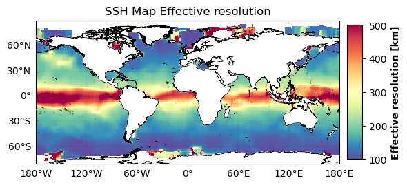
# Plot effective resolution
# Hvplot
# plot_effective_resolution(psd_output_filename)
# Matplotlib
plot_effective_resolution_png(psd_output_filename)

plot_psd_scores(psd_output_filename)

The interactive plot above allows you to explore the spectral metrics by latitude / longitude box